Mesh and Model Tools
Right clicking on the node the “Mesh and Model” option, a window will appear with the available tools (Figure 267).
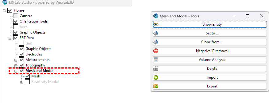
Figure 267 Mesh and Model tools panel
All the tools are described in detail in the following sections.
Show entity
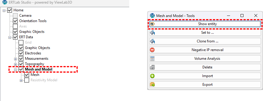
Figure 268 Show entity panel
With this command is possible to show hidden entities in the tree, like Resistivity/Conductivity/IP model. By default only resistivity is shown, and the others are hidden.
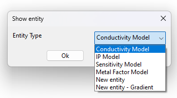
Figure 269 Entity selection
Selection a “New entity” it will be created a new Model node in the tree, with empty values (that can be filled with the commands Set to or Clone from ).
Selection a “New entity - Gradient” it will be created a new Model node in the tree, filled with values computed with “Gradient” operator, based on the model that will be selected with the window that will subsequently be shown.
Set to
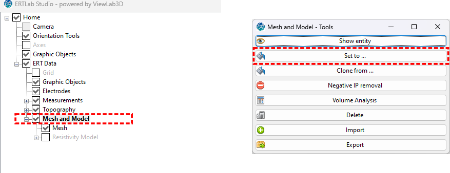
Figure 270 Set to panel
This option changes the current value of the Resistivity/Conductivity/IP model. Clicking on Set to button opens a new window for selecting the desired Entity Type through the pop-up menu (Figure 271).
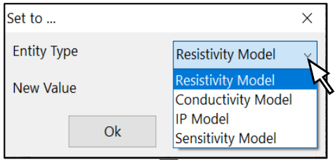
Figure 271 Example of the entity selection
Then type the desired value in the New Value number box (it is 0 by default).
It is also required to select the Method to be used.

Figure 272 Example of Resistivity Model set to 100 everywhere
Click on “Ok” to confirm.
Note
Note that after the anomaly has been added to the mesh, to see it correctly, it may be useful to adjust the position of the sections to the location of the anomaly (or in some cases it is even useful to add a Volume), or adjust the Colour Scale limits. In some cases it is also useful to view the mesh as cells, instead of the default interpolated view.
Note
Since it is obviously possible to use the “Set to” command multiple times, perhaps even using different options, it is therefore possible to update the mesh to define even very complicated models.
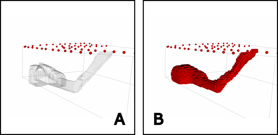
Figure 273 Example of a complex anomaly. In A the cloud of point from a laser-scan acquisition, and in B the anomaly reconstructed into the mesh.
Everywhere
the New Value specified will be set on every single cell of the mesh. The resulting mesh will be homogeneous, and the value specified will be also set as background value in the mesh generation panel.
Above/Below surface
the New Value specified will be set only to the cells that are on the half-space defined by a user-provided surface. Will be also requested a text file containing a list of the sparse points (as x y z coordinates) to be interpolated to get the surface.
Sparse bubbles
the New Value specified will be set only to the cells that are inside into user-specified spheres. Will also be requested a text file containing the list of x y z coordinates of the centre spheres, and will be also requested the radius to be used to define the size of the spheres.
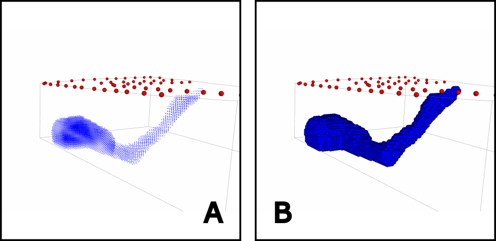
Figure 274 Example of a tricky anomaly. In A the cloud of points related the spheres that needs to be used, and in B the entire occupied volume.
Convex hull
the New Value specified will be set only to the cells that are inside the 3D shape containing the sparse cloud of point user-provided. Will also be requested a text file containing the points to be used, as a list of of x y z coordinates. Note that a Convex hull can not be concave, so the 3D shape automatically obtained from the given points will be the convex envelope that will contain all of them. If it is needed to work with a concave shape check if it is possible to subdivide it in some convex parts, or else to work with other available methods like * Sparse bubbles* or Generic (concave) 3D volume.
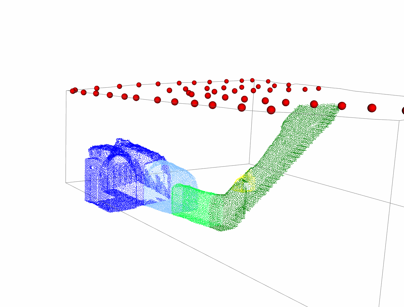
Figure 275 Example of an anomaly that needs to be subdivided in more convex parts.
Generic (concave) 3D volume
the New Value specified will be set only to the cells that are inside the 3D shape specified. The used needs to load a file containing the shape (in OBJ, STL or PLY file format). This method allows to define anomalies of even very complex shapes, and even concave shapes are here accepted.
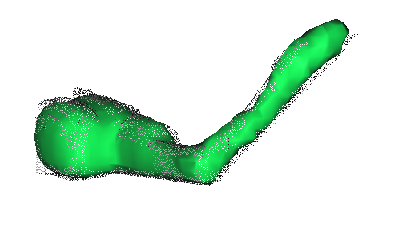
Figure 276 Example of a cloud of points describing the anomaly and the 3D shape that fits it.
The previous image is obtained thanks to CloudCompare (https://www.danielgm.net/cc/), this free tool can help on manipulating cloud of points in 3D.
Clone from
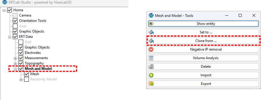
Figure 277 Clone from panel
With this command is possible to set in the current model an entity from a different node of the tree. The entities can be like Resistivity/Conductivity/IP model/…. It will be asked to specify the “Source” entity (from this or other project opened into the program) and the “Destination” entity (in the current project) where to copy the specified model.

Figure 278 Entity selection
If selection as “Destination” the “Entity” named “New” it will then added to the tree a new Model node.
Negative IP removal
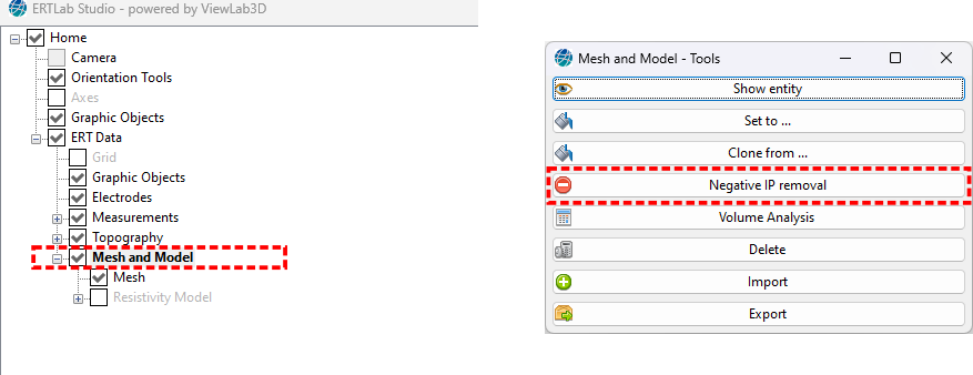
Figure 279 Negative IP removal panel
Due to computation reasons it may happen that some negative IP values will occur in the Model after the inversion processes. It is strongly recommended to delete them through the is option. It is important to not confuse these values with negative IP data, which are acceptable and manageable through the proper options (section Histogram)
Volume Analysis
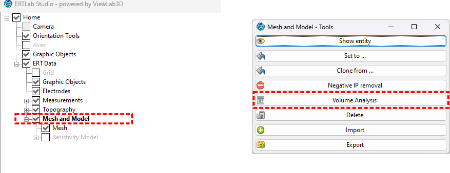
Figure 280 Volume Analysis panel
This option allows the calculation of the mesh volume (in m3 and %) and the amount of cells (in numbers and %), which have an Entity Type within a specified range. In Figure 281 the volume is calculated with the resistivity comprised between 50 and 240 Ohm*m, which correspond to 11,113.498 m3 (28.8% of the entire volume) and to 11,308 cells (28.13% of the total number of cells).
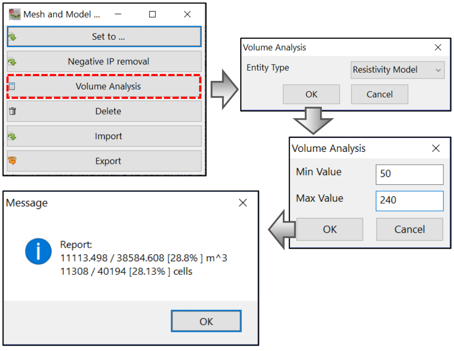
Figure 281 Volume Analysis tool
Delete
Through this option the entire mesh and model project can be deleted (to avoid accidental deletions, a confirmation window will appear).
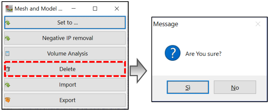
Figure 282 Delete tool
Import
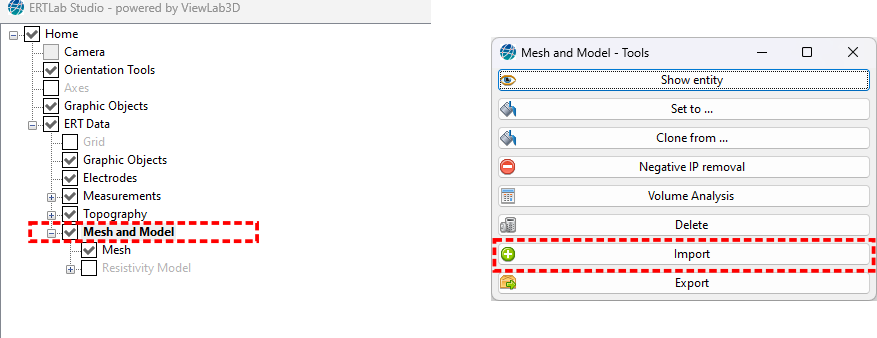
Figure 283 Import panel
Use this option to import a Mesh and/or a Model file from a DATA files (*.data or *.wDat or *.txt), a Viewer file (*.vwer), or a XYZ file (*.xyz).
Export
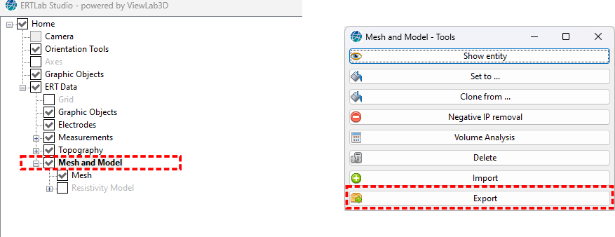
Figure 284 Export panel
Use this option to export a Resistivity/Conductivity/IP model, selecting the desired Entity Type through the pop-up menu.
If the “Foreground Only” is checked, the Background Region is not saved to reduce the necessary space. Note that it is important to export the Background Region also if the output file, after some editing, will be needed to be imported again.
It is possible to export a file as a XYZ file (.xyz) or as a EVS file (.xyz or *.fdl).
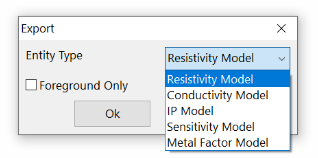
Figure 285 Export panel - choice of entity